Introduction to classification and regression with neural networks
This post covers some of the basic concepts that are necessary to understand neural networks and implement them for basic supervised classification and regression task.
The main topics are:
- What is a neural network?
- How does a neural network learn?
- Differences between classification and regression
- Implementation of neural networks for classification and regression
What is a neural network?
A neural network is a function that learns a mapping from an input $x$ and produces an output $y$:
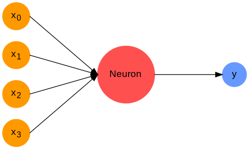
\[y = f_{\text{NN}}(x)\]The core building block that allows a neural network to learn are neurons, they have parameters that can be updated which allowing for them to learn a mapping. For a input vector $\mathbf{x}$ a neuron is defined as:
\[y = \sigma (\mathbf{w} \cdot \mathbf{x} + b)\]where $\mathbf{w}$ is a vector of trainable parameters known as the weights, $b$ a scalar value that is also trainable and known as the bias and $\sigma$ a chosen function, known as an activation function, that is normally non-linear and should be differentiable. Neurons are often depicted as nodes with inputs and outputs:
The non-linearity of activation functions is what allows an neural network to learn complex non-linear mappings. There are numerous different functions that are used but perhaps the most common is the rectified linear unit or ReLU for short. It is defined as:
\[\sigma(x)= \begin{cases} x \quad \text{if} \ x > 0 \\ 0 \quad \text{elsewhere} \end{cases}\]
Other common activations functions include TanH, Exponential Linear Unit (ELU) and Leaky ReLU. See here for more information.
From a single neuron to a network
A single neural network contains multiple neurons and they are arranged in layers.
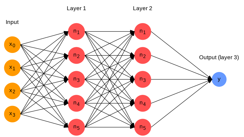
Each layer is a vector function (it returns a vector) that has a weights matrix $\mathbf{W}_{\text{l}}$ and bias vector \(\mathbf{b}_{\text{l}}\):
\[\mathbf{f}_{\text{l}}(\mathbf{x}) = \mathbf{\sigma}_{\text{l}} (\mathbf{W}_{\text{l}} \cdot \mathbf{x} + \mathbf{b}_{\text{l}})\]A neural network therefore behaves like a set of nested functions, for three layers this would be:
\[y = f_{\text{NN}} (\mathbf{x}) = \mathbf{f}_{3}(\mathbf{f}_{2}(\mathbf{f}_{1}(\mathbf{x}))\]The form of the final layer depends on the task at hand and we will focus on this later on. Now that we have an rough description of a neural network we have to understand how a neural network is trained, that is, how does it learn?
How does a neural network learn?
The answer boils down to a loss function, backpropogation and gradient descent, so what are they?
Loss function
In order for a neural network, or indeed almost any machine learning algorithm, to learn it needs a function to describe it’s current performance. This function is known as a loss function or cost function and, in the case of a supervised task, it describes the difference between the networks output and the ground truth. An example of a loss function is the mean squared error (MSE) which, for a vector of predicted values $\mathbf{\hat{y}}$ and a vector of true values $\mathbf{y}$ both of length $N$ is defined as:
\[\text{MSE} = \frac{1}{N} \sum_{i=1}^{N} (y_{i} - \hat{y}_{i})^{2}\]Such as function can then be used to update the trainable parameters of the network with an algorithm such as backpropogation.
Backpropogration and gradient descent
Backpropogation is an algorithm that calculates the gradient of the loss function with respect to the neural network’s weights. It uses the chain rule and proceeds backwards through the network from the output through all of the layers. The gradients can the be used to change the parameters and try to minimise (or maximise) the loss function.
This minimisation is then acheived using a gradient descent algorithm, such as stochastic graident descent, that explores the parameter space described by the networks weights. This is done in steps where the some data $\mathbf{x}$ is propogated through the network in a forward pass and the output $\mathbf{y}$, with the change in the loss function, used to update the weights.
For a more indepth explanation see here.
Up until this point most of statements about neural networks have been problem agnostic but now we will focus on the specifics of two common types of problems: classification and regression.
Differences between classification and regression
The main difference between classification and regression problems is what the network is trying to predict.
In classification the goal is to correctly identify the class an input corresponds to, this could be distinguishing between images of cats and dogs or between types of signals. The output is normally a predicted class or a “probability” for each of the possible classes (the sum of which is one).
For regression the goal is to predict a value (or values) given an input, for example predicting housing prices or the frequency of signal. In this case the output is continuous over some range (or potentially unbounded) and the network must output a number (or vector of numbers).
So the core difference is the output and this is reflected in the activation function used in the last layer of the network. If the output is different then the same applied the function that quantifies the “quality” of the networks output, the loss function.
Classification
The sigmoid function and binary cross-entropy
This is limited to binary classification and outputs a number in the range $[0, 1]$ that can be considered a probability:
\[\sigma(x) = \frac{1}{1 + e^{-x}}\]
The loss function for this case is binary cross-entropy (log-loss) which for $N$ samples is defined as:
\[\text{BCE} = - \sum_{i=1}^{N} y_{i} \log_{e}\left(\hat{y}_{i}\right) + (1 - y_{i}) \log_{e}\left(1 - \hat{y}_{i}\right)\]where \(\hat{y}_{i}\) is the probability for a particular sample $i$ and the $y_{i}$ the true value for the same sample.
The softmax function and cross-entropy
This is the generlised version of the sigmoid for n-class problems. The outputs are again in $[0,1]$ and importantly their sum is equal to 1. It is defined as:
\[\sigma(\mathbf{x})_{i} = \frac{e^{x_{i}}}{\sum_{j=1}^{C} e^{x_{j}}} \ \text{for} \ i=1, ..., C \ \text{and} \ \mathbf{x} \in \mathbb{R}^{C}\]where $C$ is the number of classes. The loss function is the generalised version of binary cross-entropy, cross-entropy:
\[\text{CE} = - \sum_{i=1}^{N} \sum_{j=i}^{C} y_{ij} \log_{e}(\hat{y}_{ij})\]Regression
The indentity
In regression problems the output of the neural network generally needs to be continous and unbounded so the activation function is simply the identity:
\[\sigma(x) = x\]
There is no one single loss function to use for regression task but the following are some of the most commonly used.
Mean squared error
Probably the go-to loss function for regression but is sensitive to outliers and will be heavily affected by single vey bad predictions.
\[\text{MSE} = \frac{1}{N} \sum_{i=1}^{N} (y_{i} - \hat{y}_{i})^{2}\]Mean absolute error
Very similar to MSE but not as sensitive to outliers.
\[\text{MAE} = \frac{1}{N} \sum_{i=1}^{N} |y_{i} - \hat{y}_{i}|\]Mean squared logarithmic error
The mean squared logarithmic error is well suited to problems where the values a large and you are more concerned with relative errors.
\[\text{MSLE} = \sqrt{\frac{1}{N} \sum_{i=1}^{N} \left[\log_{e}(y_{i}+1) - \log_{e}(\hat{y}_{i}+1)\right]^{2}}\]Other loss functions
The are numerous other loss functions that can be used in regression such as: root mean squared error, mean squared percentage error, R-squared… Each is best suited to particular use cases but those mentioned before will work in most situations. For more complete list see here.
Implementation of neural networks for classification and regression
Now the we’ve covered the basics we can move on to implementing a neural network. This is relatively easy in Python since there a various packages that simplify the process and save us from having to define all the core building blocks manually such as activation functions, loss functions etc. Two of the most commonly used are:
Each have their pros and cons and see use in different scenarios but at a simple level they serve the same purpose. The notebooks for this tutorial will use Keras in Tensorflow since it is supported natively in Google Colab
We start with a classification. The following notebook demonstrates how to train a neural network to classify handwritten digits from the MNIST dataset:
Classification example: 
The next notebook builds on the previous and explains how to implement a neural network for regression: